MIRA

I'm teaching a camera to tell waste apart. It's computer vision applied to a recycling problem I can actually get my hands on.

Line chart of validation mAP50 for the YOLO11n runs EXP-013 to EXP-019. The first five runs lie between 55 and 61 percent, the last two at 90.6 percent. — fig 01 Validation mAP50 across the YOLO11n runs.

Why it exists

MIRA stands for Machine Intelligence for Recycling Automation. It started with one simple question: could a cheap camera and a small model tell different kinds of waste apart well enough to help with sorting? The long-term goal is automatic sorting. The short-term goal is smaller and more useful, though. I want to find out how close the current models really are.

That's also why I'm strict about how I write about it. The project is written up as a German research paper for Jugend forscht, and I try to keep the paper and the code in step. So anything I write about a result has to say what was measured, on which data, and what it doesn't show.

How it works

MIRA is a pipeline that goes from a single photo to a live camera view. I built it in two stages, and the second one changed the project more than I expected.

Stage A: can a model tell the materials apart?

I started with photos I collected myself: 796 images in four classes. A small custom CNN came first, but then a pretrained MobileNetV2 took over. The fine-tuned MobileNetV2 reached about 87% validation accuracy, and an INT8 TFLite version kept that accuracy in a 2.6 MB file.

That was enough to show the materials could be told apart, but it left a gap. A classifier gives one label per photo. It can say "this is plastic", but a sorter also needs to know where the plastic is, and whether there are three bottles or one. That gap pushed me into stage B.

Stage B: where is the object?

Stage B moved from classification to detection. I started with YOLOv8n and then switched to YOLO11n. I trained it in Ultralytics on Kaggle and Colab T4 GPUs for 120 epochs at 640 pixels.

There are five classes: glass, metal, paper, plastic and trash. The training data is merged from four sources: TACO, TrashNet (labelled with SAM), Roboflow's Trash Detection set and a dataset by dmedhi. A script builds the final set with a fixed seed, SHA-256 de-duplication and a provenance manifest, so I can say where every image came from. The result is a class-balanced set of 6,898 images with 12,832 boxes. I dropped one source, WaRP, because adding it made the results worse. The biggest jump in accuracy came from this data work, not from changing the model.

Two good runs, two different answers

The best model depends on how you measure it, and that turned out to be the main lesson of stage B.

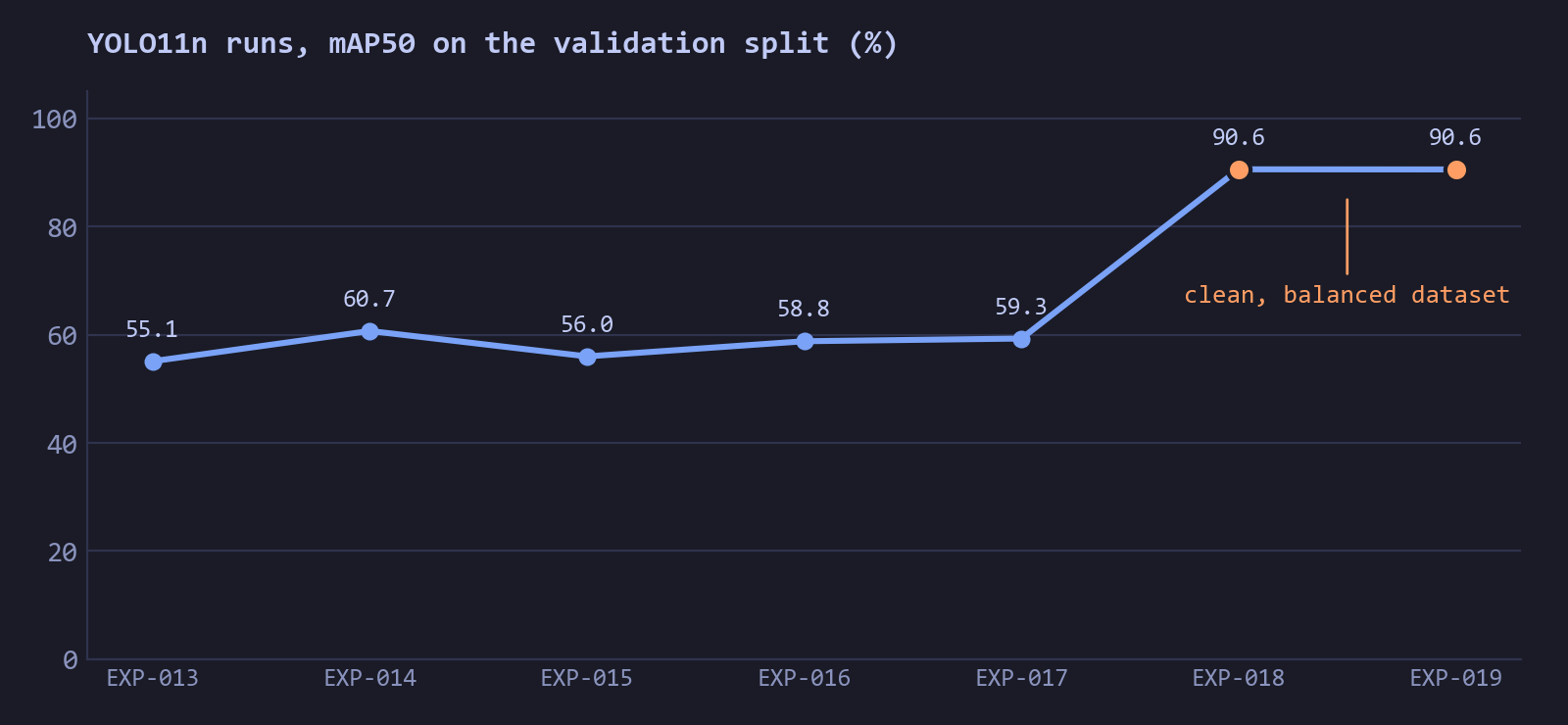
EXP-019 has the best validation numbers. It repeats EXP-018 on the clean, class-balanced dataset and reaches 90.6% mAP50 on the 415-image tabletop split. The second time, the score came out almost identical. Those are clean photos on a plain table, so the score shows the model learned that dataset well. It doesn't show how the model behaves on a real sorting belt. On real photos it didn't do badly either, though it wasn't the best model there.

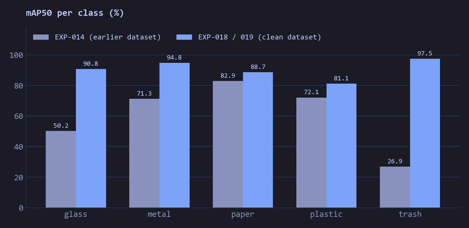
EXP-014 did best in the field benchmark, and that's the result that surprised me most. It was trained on the older mix of TACO, TrashNet and Roboflow. On its own validation split it reached only 60.7% mAP50. On the 805-image benchmark, which mixes wild and tabletop photos, it scored 85.8% image-level class-presence F1, the top result of the 11 models I tested. I put that down to the wild, mixed-background photos it was trained on. Its trash F1 was still the weakest number, at 54%. EXP-019 wasn't part of that benchmark, and the benchmark images aren't the same as the 415-image split, so I can't rank the two directly.

That gap is why I'm training again. On the tabletop split, trash reaches 97.5% mAP50, but in the field benchmark its F1 is only 54%. My guess is that a validation set of mostly easy, well-lit photos flatters the model, and that the field set is closer to what a sorter would see. I haven't proven that yet.

EXP-020 is training now. It's meant to combine the two directions: the clean, balanced data behind EXP-019's validation score, and the wild, mixed-background photos that made EXP-014 work better in the field. The goal is a model that keeps the validation score and also does well on the field benchmark. It isn't logged yet, so this page has no numbers for it.

What it does today

You can run live inference from a webcam or an IP/RTSP stream with the mira command line, with optional ByteTrack tracking.
There's a local dashboard, built with FastAPI and a web front end, that shows detections, class counts, FPS, latency, CPU and memory.
There are tools to build datasets, evaluate models and run the field benchmark. About 25 test files sit behind them.
It exports to ONNX and LiteRT/TFLite at 320 and 640 pixels. The mira-ai package on PyPI bundles the models, and the weights are on Hugging Face.

In numbers

Logged experiments: 19 (EXP-001 to EXP-019), each with its settings and result in a log; EXP-020 is in training
Field benchmark: EXP-014 at 85.8% image-level F1 (92.9% precision, 79.7% recall) on 805 images, the best of 11 models tested
Final dataset: 6,898 images and 12,832 boxes (5,108 training, 415 validation, 1,375 test)
Model: YOLO11n, 2.58 million parameters and 6.3 GFLOPs
Best validation result: 90.6% mAP50 and 82.2% mAP50-95 on the 415-image validation split, repeated in a second run at 90.58%
Before the data was rebuilt: 60.7% mAP50 (EXP-014)
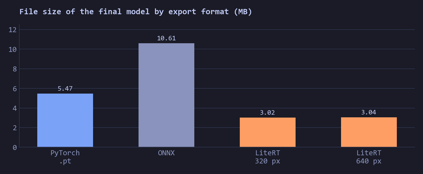
Size of the final model: 5.47 MB as PyTorch weights, 3.02 MB as a 320-pixel LiteRT file
LiteRT export, 320 pixels: 86.2% mAP50, so the smaller file loses about 4 points
Speed: 1.5 to 3.6 ms per frame on a T4 GPU; no Raspberry Pi measurement yet
Downloads: 6,500+ lifetime model downloads on Hugging Face (a download counter, not a count of people)

Figures

Bar chart of mAP50 per class, comparing the earlier dataset with the clean one: glass 50.2 to 90.8, metal 71.3 to 94.8, paper 82.9 to 88.7, plastic 72.1 to 81.1, trash 26.9 to 97.5. — fig 02 mAP50 per class, before and after the data rebuild.

Bar chart of the file size of the final model: PyTorch 5.47 MB, ONNX 10.61 MB, LiteRT at 320 pixels 3.02 MB and at 640 pixels 3.04 MB. — fig 03 File size of the final model by export format.

Where it stands

The sorting robot isn't finished, and nothing has run on a Raspberry Pi yet. EXP-020 is still training, so it doesn't have logged results yet.

The 90.6% comes from a TrashNet-style tabletop validation split, which is easy compared with a real sorting line. The 1,375-image test split hasn't been evaluated for the final runs. The field benchmark only checks whether a class is present in an image, not where it is, so it says little about detection quality. Quantized exports lose accuracy, as the 320-pixel LiteRT result shows. Crumpled paper, overlapping objects, cans seen from the opening and unusual lighting are still hard cases, and a dataset score is no guarantee for real sorting. The README also says AI tools helped with parts of the coding and debugging.